SAM SEM With Lavaan:
The Structural After Measurement Approach to SEM

by Arndt Regorz, MSc.
May 2, 2025

If you want to run an SEM model with a limited sample size, then the SAM approach to SEM can be helpful for you: SAM = structural after measurement. In this two-step (or two stages) approach, first the measurement models for the latent constructs are estimated. Then, as a second step, the structural part of the model is estimated.

First, we will look at the advantages and preconditions for an SAM model. Then you will get an R/lavaan code example for running an SAM SEM model.

Why and when SAM SEM?

In a normal SEM all parameters are estimated at the same time. The program concurrently estimates the measurement part and the structural part of the model. That has three main disadvantages:

• You need a large sample size to be able to achieve a stable estimate for all model parameters. That can lead to convergence issues in smaller samples (small relative to the model complexity).
• Possible model misspecification in the measurement part can influence the structural part of your model, leading to biased structural parameter estimates.
• The model fit information is a mixture of the measurement fit and the structural fit. In most cases the measurement model has more parameters; thus the fit indices primarily reflect the fit of the measurement model, even though in many cases you are primarily interested in the structural model of the SEM.

Contrast that with the estimation process in an SAM SEM:

First, the measurement parts of the model are estimated. You can decide how many different measurement models should be estimated. The two most extreme options are: One separate measurement model for each factor; one combined measurement model for all factors. In general, it is better to have separate measurement models for different constructs, unless, e.g., those are connected (by cross-loadings, error covariances).

Second, the structural part of the model is estimated, using the results of the first step.

This has clear advantages:

• For each part of the model estimation (measurement models, structural model) the ratio between the number of observations and the estimated parameters is higher leading to more stable results.
• The estimation is more robust against local misspecification.
• You get separate fit indices for the measurement part and the structural part of the model. That is important since most often you are primarily interested in the structural part.

When should you use SAM SEM?

In general, it is helpful to use if you have many constructs and only a moderate sample size. However, the SAM SEM approach is not designed to investigate possible model misspecification in the measurement part of the model. For that reason you should either use it with established scales with well known psychometric properties or you should run conventional CFAs to make sure that the measurement models work as designed, before running your SAM SEM.

Lavaan code for SAM SEM

library(lavaan)

For this example I have used the dataset PoliticalDemocracy that comes as part of lavaan. Since there are only 75 observations this dataset is a bit too small for a conventional SEM estimation, making it an ideal use case for SAM SEM.

Figure 1

Model Specification Political Democracy

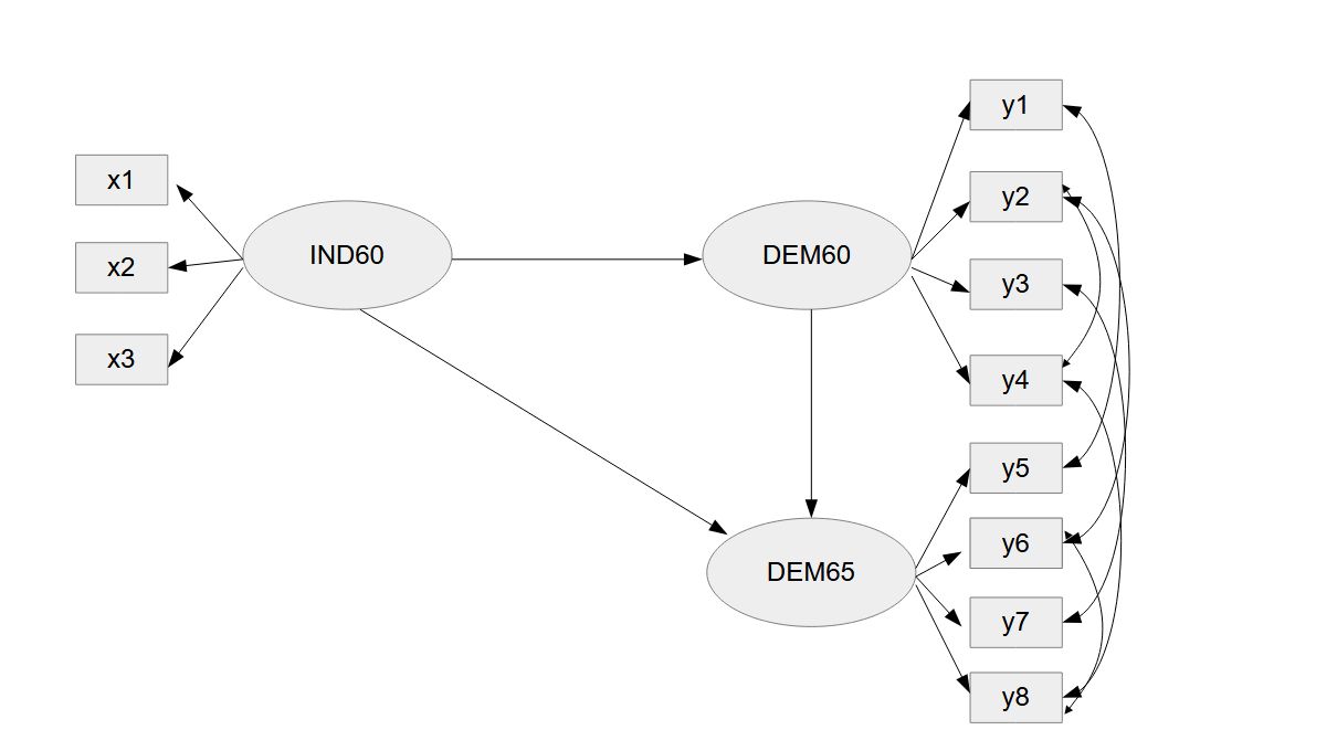
The specification of the model is the same as in a conventional SEM.

model <- '
ind60 =~ x1 + x2 + x3
dem60 =~ 1 * y1 + l2 * y2 + l3 * y3 + l4 * y4
dem65 =~ 1 * y5 + l2 * y6 + l3 * y7 + l4 * y8

dem60 ~ ind60
dem65 ~ ind60 + dem60

y1 ~~ y5
y2 ~~ y6
y3 ~~ y7
y4 ~~ y8
y2 ~~ y4
y6 ~~ y8 '

What is new is the estimation part of the model:

fit.sam <- sam(model,
data = PoliticalDemocracy,
cmd ="sem",
se = "twostep",
mm.list = list(ind = "ind60", dem = c("dem60", "dem65")),
sam.method = "local")

Here, we use the sam function in order to estimate the SAM SEM. Then we have, as always, the model specification and the dataframe.

The parameter cmd defines what kind of lavaan model is to be estimated. The most common choices are “sem” and “cfa”.

The parameter se = “twostep” requests two-step standard errors. This is important because we have two possible sources of random variation in the model: The measurement part and the structural part. The two-step standard error takes the variation in the first step into account when calculating the standard errors for the second step, the structural part. That leads to correcter test statistics and p-values for the structural part of the model.

The key ingredient of the sam function is the parameter mm.list. Here the separate blocks in the measurement model are specified. In this example there are two blocks: ind (industrialization) and dem (democracy).

In general one should specify one measurement block for each construct unless there are reasons to combine two or more constructs into one block. And one of the key reasons for that is that two or more blocks have shared elements in their measurement model. In this example there are error covariances connecting the items of dem60 and dem65. For that reason it would make no sense to estimate those two measurement models separately from each other. Other possible reasons for combined measurement models are cross loadings or constructs with only two items (that would be underidentified if estimated in isolation).

There are different SAM methods, in general I would use the method “local”. For more information about this decision see Rosseel and Loh (2024).

If you had missing data, then you could add missing = "FIML".

After the estimation we use the summary function on the resulting fit object.

summary(fit.sam,
standardized = T,
remove.step1 = F)

There is one parameter not used in standard SEM: remove.step1. As a default you will get only detailed results for step 2, the structural part of the model. However, I like to see the results for the measurement blocks as well.

In the output, first we get some general information about the model. That is followed by summary information about the measurement part of the model:

Summary Information Measurement + Structural:

Block Latent Nind Chisq Df
1 ind60 3 0.00 0
2 dem60,dem65 8 15.32 16

For each measurement block you get the chi-square and the degrees of freedom. Since the measurement model for the variable ind60 was just identified here we get a perfect fit. If you want to calculate the p-value from the test statistic and degree of freedom, here for the block dem with the two constructs dem60 and dem65, you can use this r code:

pchisq(15.32, 16, lower.tail = F)

As a result we get a p-value of .501, indicating good fit.

Then, you get reliability information (similar to McDonald’s omega) for the constructs:

Model-based reliability latent variables:

ind60 dem60 dem65
0.966 0.868 0.87

This is followed by the summary information for the structural part:

Summary Information Structural part:

chisq df cfi rmsea srmr
0 0 1 0 0

Since in this example we have a just-identified structural model (df = 0) we get a perfect fit.

After that you get the parameter estimates. The output looks the same as in a normal SEM with one exception: For each parameter you get the information in which part (1: measurement, 2: structural) of the estimation process it was calculated.

Parameter Estimates:

Standard errors Twostep
Information Expected
Information saturated (h1) model Structured

Latent Variables:
Step Estimate Std.Err z-value P(>|z|) Std.lv Std.all
ind60 =~
x1 1 1.000 0.667 0.917
x2 1 2.193 0.142 15.403 0.000 1.464 0.976
x3 1 1.824 0.153 11.883 0.000 1.217 0.872
dem60 =~
y1 1 1.000 2.170 0.845
y2 (l2) 1 1.213 0.143 8.483 0.000 2.631 0.692
y3 (l3) 1 1.210 0.125 9.690 0.000 2.626 0.762
y4 (l4) 1 1.273 0.122 10.453 0.000 2.761 0.839
dem65 =~
y5 1 1.000 2.128 0.803
y6 (l2) 1 1.213 0.143 8.483 0.000 2.580 0.762
y7 (l3) 1 1.210 0.125 9.690 0.000 2.575 0.817
y8 (l4) 1 1.273 0.122 10.453 0.000 2.708 0.833

Regressions:
Step Estimate Std.Err z-value P(>|z|) Std.lv Std.all
dem60 ~
ind60 2 1.454 0.389 3.741 0.000 0.447 0.447
dem65 ~
ind60 2 0.558 0.225 2.480 0.013 0.175 0.175
dem60 2 0.871 0.076 11.497 0.000 0.888 0.888

Covariances:
Step Estimate Std.Err z-value P(>|z|) Std.lv Std.all
.y1 ~~
.y5 1 0.577 0.364 1.585 0.113 0.577 0.266
.y2 ~~
.y6 1 2.068 0.733 2.822 0.005 2.068 0.344
.y3 ~~
.y7 1 0.727 0.611 1.190 0.234 0.727 0.180
.y4 ~~
.y8 1 0.476 0.453 1.049 0.294 0.476 0.148
.y2 ~~
.y4 1 1.390 0.685 2.030 0.042 1.390 0.283
.y6 ~~
.y8 1 1.257 0.583 2.156 0.031 1.257 0.319

Variances:
Step Estimate Std.Err z-value P(>|z|) Std.lv Std.all
.x1 1 0.084 0.020 4.140 0.000 0.084 0.159
.x2 1 0.108 0.074 1.455 0.146 0.108 0.048
.x3 1 0.468 0.091 5.124 0.000 0.468 0.240
.y1 1 1.879 0.431 4.355 0.000 1.879 0.285
.y2 1 7.530 1.363 5.523 0.000 7.530 0.521
.y3 1 4.966 0.966 5.141 0.000 4.966 0.419
.y4 1 3.214 0.722 4.449 0.000 3.214 0.297
.y5 1 2.499 0.518 4.824 0.000 2.499 0.356
.y6 1 4.809 0.924 5.202 0.000 4.809 0.419
.y7 1 3.302 0.699 4.722 0.000 3.302 0.332
.y8 1 3.227 0.720 4.482 0.000 3.227 0.306
ind60 2 0.446 0.087 5.135 0.000 1.000 1.000
.dem60 2 3.766 0.848 4.439 0.000 0.800 0.800
.dem65 2 0.189 0.224 0.843 0.399 0.042 0.042

References

Rosseel, Y. (2024). The ‘Structural After Measurement’ (SAM) approach to SEM [slides]. The Joint Quantitative Brownbag (JQBB) Speaker Series. https://users.ugent.be/~yrosseel/lavaan/slides/rosseel_jqbb2024.pdf
(Seem to be unavailable - try archive.org)

Rosseel, Y., & Loh, W. W. (2024). A structural after measurement approach to structural equation modeling. Psychological Methods, 29(3), 561–588. https://doi.org/10.1037/met0000503

Citation

Regorz, A. (2025, May 4). SAM SEM with lavaan: The structural after measurement approach to SEM. Regorz Statistik. https://www.regorz-statistik.de/blog/lavaan_sam_sem.html