Outlier in a Lavaan Model:
Identifying Influential Cases

by Arndt Regorz, MSc.
April 21, 2026

If you run a confirmatory factor analysis (CFA) or a structural equation model (SEM) you will want to check for outliers or influential cases since these can meaningfully impact the results of your analysis. This tutorial shows you how to do that for a lavaan model using the semfindr package.

Influential Cases

In a regression analysis there are many different approaches to identify outliers or influential cases.

A popular approach to identify influential cases in a regression context is called DFBETA. This identifies cases that have a huge impact on the resulting regression slopes.

DFBETA is based on the leaving-one-out approach (LOO). The model is refit once for each observation, each time omitting that case from the data. This way it is possible to assess the impact of a single observation: How does the regression slope change without that observation?

The semfindr package in R has made this approach available for SEM, CFA and path analysis with lavaan, too.

Identifying Influential Cases With the semfindr Package

First, we need to install the semfindr package (once) and load it (each session we want to use it).

#install.packages("semfindr")
library(semfindr)

Then we run our lavaan model, in this example a three-factor CFA.

library(lavaan)

head(HolzingerSwineford1939_influential_case_introduced, 5)

cfa_model <- '
visual =~ x1 + x2 + x3
language =~ x4 + x5 + x6
speed =~ x7 + x8 + x9
'

model_fit <- cfa(model = cfa_model,
data = HolzingerSwineford1939_influential_case_introduced,
std.lv = T)

summary(model_fit,
standardized = T)

standardizedsolution(model_fit, level=.95) # Confidence interval for beta

After that we can start identifying influential cases.

# INFLUENTIAL CASES

This starts with rerunning the lavaan model as many times as we have observations in our sample (= LOO approach).

# 0 Rerun this model (leaving one out - LOO)

fit_rerun <- lavaan_rerun(model_fit)

With a simple model and a small dataset that takes a couple of seconds. With a more complicated model and a larger dataset, however, this can take quite some time.

In that case it is helpful to use parallel processing. Most modern computers have more than one core. You can get this information somewhere in the system information of your computer (in the case of Windows you open the Task Manager, go to the Performance tab and check the specifications for CPU).

My computer has 4 cores; thus I use this code:

fit_rerun <- lavaan_rerun(model_fit,
parallel = T,
ncores = 4) # faster with parallel processing

There are different measures of parameter change. DFTHETAS is a standardized change measure, i.e. change standardized with the standard error of the parameter. Unfortunately, this measure is quite difficult to interpret. The results are ordered by the general Cook's distance.

# 1 Standardized change (DFTHETAS)

change_est <- est_change(fit_rerun)
change_est

--- visual~~language visual~~speed language~~speed gcd
100 -1.130 0.531 -0.537 3.191
85 0.184 0.026 0.000 2.190
87 -0.897 0.079 -0.120 1.612
32 0.369 0.243 0.176 1.209
40 -0.181 0.203 0.352 1.119
1 0.131 -0.018 0.019 1.098
19 0.308 0.264 0.264 1.089
36 0.196 0.076 0.057 0.985
26 0.350 0.070 0.072 0.757
2 -0.031 0.058 -0.051 0.734

Easier to interpret is the raw parameter change of the standardized parameter estimates, DFZTHETA. This tells you how much the standardized parameter (beta) has been influenced by one observation.

# 2 Raw parameter change standardized (DFZTHETA)

change_est_raw_s <- est_change_raw(fit_rerun,
standardized = T)
change_est_raw_s

You can limit the output to a specific type of parameters. For example, here we only look at the variances and covariances:

change_est_raw_vk <- est_change_raw(fit_rerun,
parameters = ("~~"),
standardized = T)
change_est_raw_vk

You can limit the output further by limiting it to specific parameters. For example, here to three factor correlations:

change_est_raw_k <- est_change_raw(fit_rerun,
parameters = c("visual~~language", "visual~~speed", "language~~speed"),
standardized = T)
change_est_raw_k

-- id visual~~language id visual~~speed id language~~speed
1 100 -0.132 100 0.075 100 -0.066
2 87 -0.105 7 -0.066 43 0.044
3 32 0.046 83 -0.060 40 0.043
4 26 0.042 19 0.035 70 0.042
5 90 -0.040 32 0.033 19 0.031
6 19 0.038 99 0.032 50 0.030
7 11 0.037 25 -0.029 32 0.021
8 76 -0.034 40 0.028 3 -0.020
9 72 -0.031 37 0.025 67 -0.020
10 86 -0.030 9 0.023 7 -0.020

The first value for visual~~ language can be interpreted like this: The case with the id=100 has resulted in a correlation between visual and language that is .132 smaller than in a sample without that case. Without case 100 this correlation would be higher.

A possible cut-off value for influential cases is .10. The reasoning behind that is that for standardized parameters (correlations) .20 is the difference between small (.10) and medium (.30) or between medium and large (.50). Thus .10 is 50% of such a difference.

You can also look at the change im model fit that is due to one observation.

# 3 Change in model fit

change_fit <- fit_measures_change(fit_rerun)
print(change_fit,
sort_by = "cfi")

--- chisq cfi rmsea tli
100 -3.694 0.017 -0.013 0.026
99 3.481 -0.014 0.016 -0.020
85 2.973 -0.012 0.013 -0.018
14 -2.586 0.010 -0.010 0.015
8 -2.172 0.009 -0.008 0.013
1 1.836 -0.008 0.008 -0.012
13 -1.890 0.008 -0.007 0.012
23 -1.829 0.008 -0.007 0.011
26 1.975 -0.008 0.008 -0.011
79 -1.855 0.007 -0.007 0.011

Note:
- Only the first 10 case(s) is/are displayed. Set ‘first’ to NULL to display all cases.
- Cases sorted by cfi in decreasing order on absolute values.

A possible cut-off is a chisq change of 10 (often used for modification indices) or a cfi change of .01 (often used in measurement equivalence testing).

And finally, you can plot influential cases based on the generalized Cook's distance (gcd).

# 4 Plot influence cooks distance

gcd_plot(influence_stat(fit_rerun),
largest_gcd = 5)

A possible cut-off value is a gcd larger than 1.

You can limit that to those parameters that are of theoretical value for you, for instance the factor correlations in our example.

gcd_plot(influence_stat(fit_rerun,
parameters = c("visual~~language", "visual~~speed", "language~~speed")),
largest_gcd = 5)

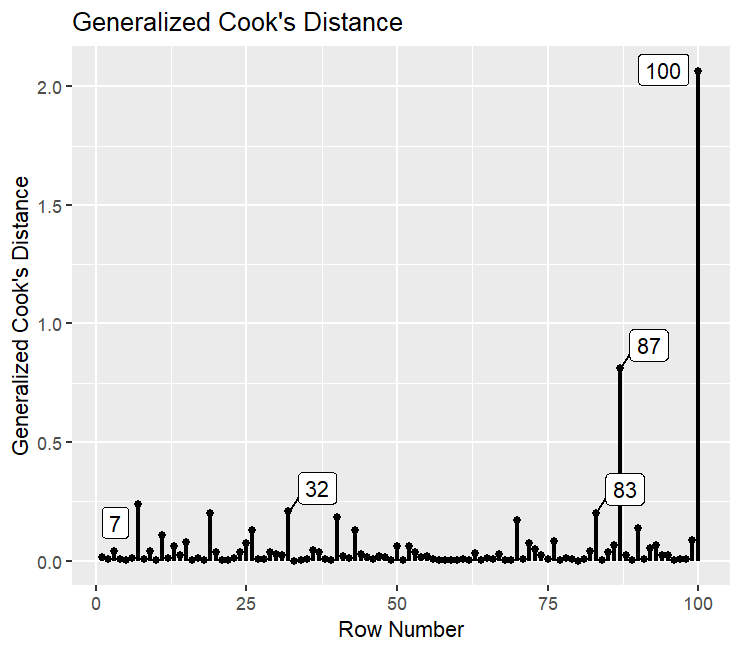
Here we can see that only one case, no. 100, has a larger gcd than 1 if we only look at the parameters that are theoretically relevant for us.

What to Do With Influential Cases?

If you have identified one or more influential cases, then the question remains: What to do with these cases? There are different possible answers to that.

One possible approach is to manually inspect those extreme observations and decide whether they represent a legitimate (but extreme) answer or whether they are the result of errors or of participants not answering in earnest (e.g., giving the same answer for each question). In that case one would retain the legitimate cases.

A second possible approach is to run a sensitivity analysis: Analyzing your CFA or SEM at first with all cases and a second time without the extreme cases. If the key results of your analysis stay the same, then you know that the extreme cases don't have an undue influence on the overall results for you hypotheses.

References

Cheung, S. F., & Lai, M. H. (2026). semfindr: An R package for identifying influential cases in structural equation modeling. Multivariate Behavioral Research. Advance online publication. https://doi.org/10.1080/00273171.2026.2634293

Citation