How to interpret a Collinearity Diagnostics table in SPSS

Arndt Regorz, Dipl. Kfm. & M.Sc. Psychologie, 01/18/2020

If the option "Collinearity Diagnostics" is selected in the context of multiple regression, two additional pieces of information are obtained in the SPSS output.

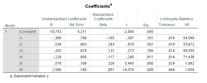
First, in the "Coefficients" table on the far right a "Collinearity Statistics" area appears with the two columns "Tolerance" and "VIF".

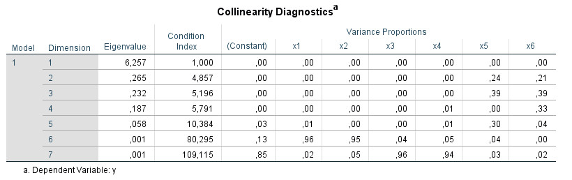
And below this table appears another table with the title "Collinearity Diagnostics":

The interpretation of this SPSS table is often unknown and it is somewhat difficult to find clear information about it. The following tutorial shows you how to use the "Collinearity Diagnostics" table to further analyze multicollinearity in your multiple regressions. The tutorial is based on SPSS version 25.

1. YouTube Video-Tutorial

(Note: When you click on this video you are using a service offered by YouTube.)

2. Column "Dimension"

Let us start with the first column of the table. Similar but not identical to a factor analysis or PCA (principle component analysis), an attempt is made to determine dimensions with independent information. More precisely, a singular value decomposition (Wikipedia, n.d.) of the X matrix is apparently performed without its prior centering (Snee, 1983).

3. Column "Eigenvalue"

Several eigenvalues close to 0 are an indication for multicollinearity (IBM, n.d.). Since "close to" is somewhat imprecise it is better to use the next column with the Condition Index for the diagnosis.

4. Column "Condition Index"

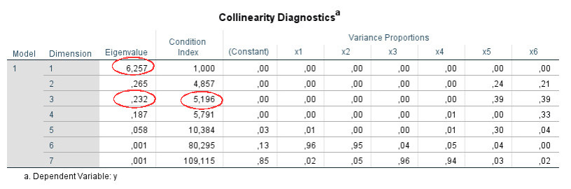
These are calculated from the eigenvalues. The condition index for a dimension is derived from the square root of the ratio of the largest eigenvalue (dimension 1) to the eigenvalue of the dimension. image Condition index collinearity diagnostics SPSS

In the table above, for example, for dimension 3:
Eigenvalue dim 1: 6.257
Eigenvalue dim 3: 0.232
Eigenvalue dim 1 / Eigenvalue dim 3: 26.970
Square root (=Condition Index): 5.193
(the difference to the output 5.196 is due to rounding error)

More important than the calculation is the interpretation of the Condition Index. Values above 15 can indicate multicollinearity problems, values above 30 are a very strong sign for problems with multicollinearity (IBM, n.d.). For all lines in which correspondingly high values occur for the Condition Index, one should then consider the next section with the "Variance Proportions".

5. Section "Variance Proportions"

Next, consider the regression coefficient variance-decomposition matrix. Here for each regression coefficient its variance is distributed to the different eigenvalues (Hair, Black, Babin, &Anderson, 2013). If you look at the numbers in the table, you can see that the variance proportions add up to one column by column.

According to Hair et al. (2013) for each row with a high Condition Index, you search for values above .90 in the Variance Proportions. If you find two or more values above .90 in one line you can assume that there is a collinearity problem between those predictors. If only one predictor in a line has a value above .90, this is not a sign for multicollinearity.

However, in my experience this rule does not always lead to the identification of the collinear predictors. It is quite possible to find multiple variables with high VIF values without finding lines with pairs (or larger groups) of predictors with values above .90. In this case I would also search for pairs in a line with variance proportion values above .80 or .70, for example.

6. Hierarchical regression

If you perform a hierarchical regression, the corresponding values of the "collinearity diagnostics" table appear separately for each regression step ("Model 1", "Model 2"):

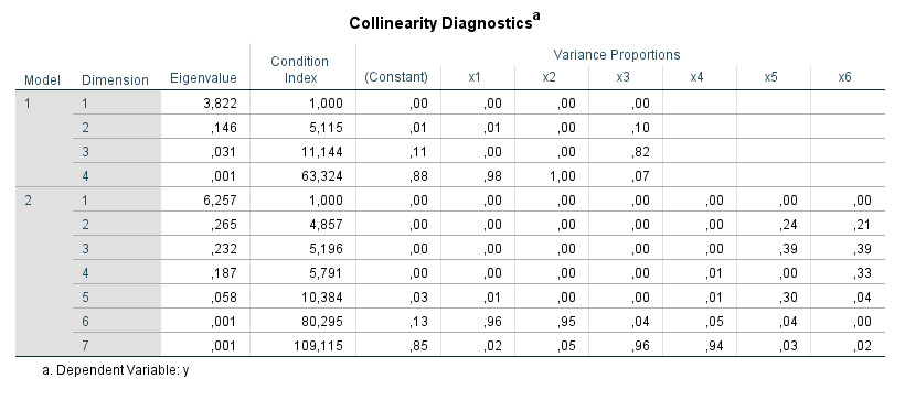
Table Collinearity diagnostics hierarchical regression

I would primarily interpret the data for the last step or, in general, the data for those steps that you report and interpret for your hypothesis tests in more detail.

7. How to use the information

When I want to analyze a multiple regression output for multicollinearity, this is how I proceed:

I look at the value "VIF" in the table "Coefficients". If this value is less than 10 for all predictors the topic is closed for me.
If there are only a maximum of two values of the VIF above 10, I assume that the collinearity problem exists between these two values and do not interpret the "collinearity diagnostics" table. However, if there are more than two predictors with a VIF above 10, then I will look at the collinearity diagnostics.
I identify the lines with a Condition Index above 15.
In these lines I check if there is more than one column (more than one predictor) with values above .90 in the variance proportions. In this case I assume a collinearity problem between the predictors that have these high values.
If only one predictor in a line has a high value (above .90), this is not relevant to me.
If I have not been able to identify the source of the multicollinearity yet, because there are no lines with several variance proportions above .90, I reduce this criterion and consider, for example, pairs of predictors (or groups of predictors) with values above .80 or .70 as well.

8. Example

Step 1: There are predictors with a VIF above 10 (x₁, x₂, x₃, x₄).

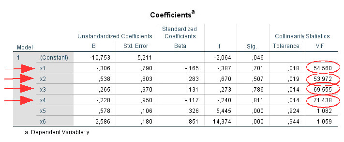
SPSS Collinearity statistics example VIF

Step 2: There are more than two predictors (here: four) to which this applies. Therefore look at the collinearity diagnostics table:

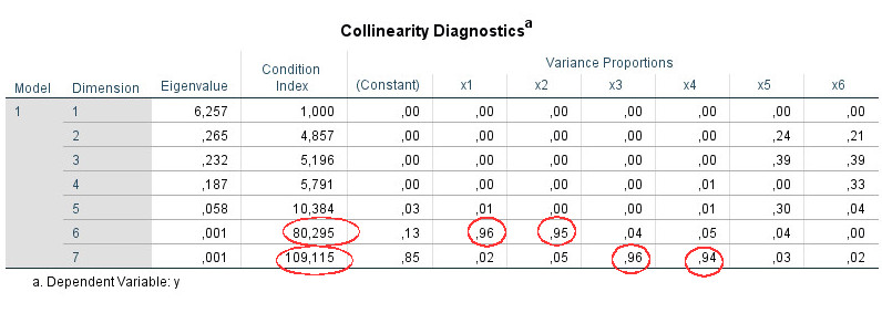
SPSS Collinearity diagnostics table example

Step 3: Dimensions 6 and 7 show a condition index above 15.

Step 4: For each of the two dimensions search for values above .90. For dimension 6 we find these for the predictors x₁ and x₂, for dimension 7 for the predictors x₃ and x₄. On this basis you assume that there are actually two different collinearity problems in your model: between x₁ and x₂ and between x₃ and x₄. (However, if all values above .90 for these four predictors had been on one line, that would have indicated a single multicollinearity problem of all four variables).

Steps 5 and 6 are not used in this example because we have already identified the sources for collinearity.

9. References

Hair, J. F., Black, W. C., Babin, B. J., & Anderson, R. E. (2013). Multivariate data analysis: Advanced diagnostics for multiple regression [Online supplement]. Retrieved from http://www.mvstats.com/Downloads/Supplements/Advanced_Regression_Diagnostics.pdf

IBM (n.d.). Collinearity diagnostics. Retrieved August 19, 2019, from https://www.ibm.com/support/knowledgecenter/en/SSLVMB_23.0.0/spss/tutorials/reg_cars_collin_01.html

Snee, R. D. (1983). Regression Diagnostics: Identifying Influential Data and Sources of Collinearity. Journal of Quality Technology, 15, 149-153. doi:10.1080/00224065.1983.11978865

Wikipedia (n.d.). Singular value decomposition. Retrieved August 19, 2019, from https://en.wikipedia.org/wiki/Singular_value_decomposition