SEM/CFA: Be Careful With the Z-Test

by Arndt Regorz, MSc.
May 5, 2024

If you want to test a parameter in an SEM or a CFA then in most cases you will find a Z-test in the output.

Should you use the Z-test for testing your hypotheses? This blogpost shows you the problems with this test, and what test you can use instead.

This problem concerns SEM-programs in general.

The specific example I have used here was written in R. If you want to try it out yourself then you can find the R code in the appendix at the end of this blog post.

1. Z-test - The Default Option

After successfully running a confirmatory factor analysis (CFA) or a structural equation model (SEM) in most cases you want to test your hypotheses, looking at the test results for specific parameters, e.g., for structural paths in an SEM or for factor correlations in a CFA.

In the output of your SEM program you most likely will find results of a Z-test. In lavaan it is a column called “z-value”, in AMOS a column called “C.R.” (for critical ratio). This is accompanied by a column with p-values.

Here is an example from lavaan. It is a simple SEM model with three latent variables. For each latent variable the loading of the first item was constrained to one (default option for model identification purposes).

Figure 1

SEM Results With First Loading Constrained to One

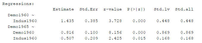
An output like this is often used to decide whether to confirm one’s hypotheses, based on the p-values. And, quite often, instead of the unstandardized estimates (“Estimate”) the fully standardized betas (here: “Std.all”) are reported.

2. Z-test - The Scale Matters

The problem with this approach is this: These results of the parameter tests can change with changes in the factor scale (i.e., with changes in the latent variable identification method).

That is different from what you may be used to with regression analysis, where changes in the metric have no influence on the test statistics and p-values. The reason for this difference is that an ordinary regression is linear. But fitting a CFA or an SEM is not a linear process even though those are linear models.

Let’s see what happens when we change the identification method and thereby the metric for the latent variables in the example above.

For the reported example the loading for the first indicator of each factor was set to 1 (default method in most SEM programs).

If instead the loading for the second indicator of each factor is set to 1, then the resulting overall model fit (chi-square test) is the same. But the test statistics for the structural paths are different:

Figure 2

SEM Results With Second Loading Constrained to One

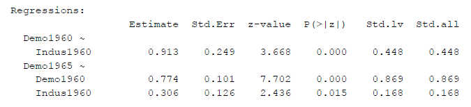
We get different Z-values, but in this case only minor differences so it does not change the p-values (e.g. z-value for the first regression path 3.668 instead of 3.728).

As a third option we could constrain the latent variable variances to 1 and freely estimate all loadings (the preferred option in many CFAs). Then we get different z-values, too:

Figure 3

SEM Results With Factor Variance Constrained to One

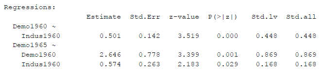
Now, even the p-values are different (for the path from Indus1960 to Demo1965, p = .029 instead of p = .015 in the other two identification methods - with the same data and the same basic model!).

It can be easily imagined that, other than in this example, a path gets a significant result with one identification/scaling method and an insignificant result with another scaling method.

This is not good!

One could change the hypothesis test results of such a model simply by trying out different scaling methods (You should not do that!). Results obtained from the z test become somewhat questionable due to this problem.

3. No Test for the Betas

Another problem is, that the Z-values and p-values apply only to the unstandardized estimates, not to the standardized estimates (i.e., the betas). That can be easily seen in the output examples above. The standardized results (last column, “Std.all”) are the same for all three different scaling methods. But the Z-values are different. Obviously, one and the same standardized estimate can’t have different Z-values and possibly different p-values at the same time. From this it can be seen that we don’t have p-values for the standardized results in the output above.

In general, it would be wrong to report the standardized results together with the p-values of the unstandardized estimates, even though this happens a lot in reality.

There is an exception to that: Some programs (e.g., Mplus, as far as I know) are able to provide separate test statistics and p-values for standardized estimates. Then, you could report standardized estimates and their p-values.

4. The Alternative: Likelihood-Ratio Test

Luckily, there is an alternative to the Z-test that does not have this problem: A likelihood-ratio test (LR test, chi-square difference test). With the LR-test you compare two models:

The first model is the model you have hypothesized.
The second model is a model where the parameter for which you want a p-value is constrained to zero.

Then you run the LR test comparing the two models. As a result you get a chi-square test statistic and a p-value for the comparison between both models. And this result does not depend on the metric or identification method you are using.

Here are the test results for testing the path Indus1960 to Demo1965 with an LR-test:

Scaling by setting the first loading for each factor to one
Chi-square (df = 1) = 5.569, p = .01828

Scaling by setting the second loading for each factor to one
Chi-square (df = 1) = 5.569, p = .01828

Scaling by setting the latent variable variances to one
Chi-square (df = 1) = 5.569, p = .01828

Regardless of the identification method, now we get the same results!

And since fully standardized results are based on a specific scale, too, the p-values derived from a LR test are correct for standardized results (betas) as well.

There is one limitation to this approach. Sometimes you want to test a parameter in a part of the model that is just identified. Then constraining one parameter to 0 could lead to underidentification, making it impossible to estimate the constrained model.

Example: You have a very simple CFA with one factor and three indicator variables. If you wanted to test the significance of a factor loading with a LR test then this would not work. Because in the constrained version of the model you would have only two indicators for the factor and that is an underidentified model.

Conclusion

You should not use the Z-test for the main results (i.e., for the tests of your hypotheses) of your study. Instead, you should report p-values based on LR-tests (Gonzalez & Griffin, 2001).

And you should not report the p-values derived from a Z-test for unstandardized results together with betas (standardized results). Instead, either give p-values specifically for the standardized results (if your SEM software is able to provide them) or report results from a LR-test for the betas.

Reference

Gonzalez, R., & Griffin, D. (2001). Testing parameters in structural equation modeling: Every "one" matters. Psychological Methods, 6(3), 258-269.

Citation

Regorz, A. (2024, May 5). SEM/CFA: Be careful with the z-test. Regorz Statistik. http://www.regorz-statistik.de/blog/be_careful_with_the_z_test.html

Appendix: R-Code for This Tutorial

Here is the R code that has been used to get the results reported above. The dataset used is part of lavaan, so you can directly run this code in r as long as you have installed the lavaan package:

library(lavaan)

# 1 Testing parameters with Z-test

# 1a Identification 1st item

struct_model_1a <- '
# Loadings
Indus1960 =~ x1 + x2 + x3
Demo1960 =~ y1 + y2 + y3 + y4
Demo1965 =~ y5 + y6 + y7 + y8

# Structural Model
Demo1960 ~ Indus1960
Demo1965 ~ Demo1960 + Indus1960

#Covariances
y1 ~~ y5
y2 ~~ y6
y3 ~~ y7
y4 ~~ y8
'

model_fit_1a <- sem(data = PoliticalDemocracy,
model = struct_model_1a)

summary(model_fit_1a, fit.measures = TRUE,
standardized = TRUE)

# 1b Identification 2nd item

struct_model_1b <- '
# Loadings
Indus1960 =~ NA * x1 + 1 * x2 + x3
Demo1960 =~ NA *y1 + 1 * y2 + y3 + y4
Demo1965 =~ NA *y5 + 1 * y6 + y7 + y8

# Structural Model
Demo1960 ~ Indus1960
Demo1965 ~ Demo1960 + Indus1960

#Covariances
y1 ~~ y5
y2 ~~ y6
y3 ~~ y7
y4 ~~ y8
'

model_fit_1b <- sem(data = PoliticalDemocracy, model = struct_model_1b)

summary(model_fit_1b, fit.measures = TRUE, standardized = TRUE)

# 1c Identification Factor Variances

struct_model_1c <- '
# Loadings
Indus1960 =~ x1 + x2 + x3
Demo1960 =~ y1 + y2 + y3 + y4
Demo1965 =~ y5 + y6 + y7 + y8

# Structural Model
Demo1960 ~ Indus1960
Demo1965 ~ Demo1960 + Indus1960

#Covariances
y1 ~~ y5
y2 ~~ y6
y3 ~~ y7
y4 ~~ y8
'

model_fit_1c <- sem(data = PoliticalDemocracy,
model = struct_model_1c, std.lv = TRUE)

summary(model_fit_1c, fit.measures = TRUE,
standardized = TRUE)

# 2 LR-Test

# 2a

struct_model_2a <- '
# Loadings
Indus1960 =~ x1 + x2 + x3
Demo1960 =~ y1 + y2 + y3 + y4
Demo1965 =~ y5 + y6 + y7 + y8

# Structural Model
Demo1960 ~ Indus1960
Demo1965 ~ Demo1960 + 0 * Indus1960

#Covariances
y1 ~~ y5
y2 ~~ y6
y3 ~~ y7
y4 ~~ y8
'

model_fit_2a <- sem(data = PoliticalDemocracy,
model = struct_model_2a)

lavTestLRT(model_fit_1a, model_fit_2a)

# 2b

struct_model_2b <- '
# Loadings
Indus1960 =~ NA * x1 + 1 * x2 + x3
Demo1960 =~ NA *y1 + 1 * y2 + y3 + y4
Demo1965 =~ NA *y5 + 1 * y6 + y7 + y8

# Structural Model
Demo1960 ~ Indus1960
Demo1965 ~ Demo1960 + 0 * Indus1960

#Covariances
y1 ~~ y5
y2 ~~ y6
y3 ~~ y7
y4 ~~ y8
'

model_fit_2b <- sem(data = PoliticalDemocracy,
model = struct_model_2b)

lavTestLRT(model_fit_1b, model_fit_2b)

# 2c

struct_model_2c <- '
# Loadings
Indus1960 =~ x1 + x2 + x3
Demo1960 =~ y1 + y2 + y3 + y4
Demo1965 =~ y5 + y6 + y7 + y8

# Structural Model
Demo1960 ~ Indus1960
Demo1965 ~ Demo1960 + 0 * Indus1960

#Covariances
y1 ~~ y5
y2 ~~ y6
y3 ~~ y7
y4 ~~ y8
'

model_fit_2c <- sem(data = PoliticalDemocracy,
model = struct_model_2c, std.lv = TRUE)

lavTestLRT(model_fit_1c, model_fit_2c)