R - Moderation Analysis with PROCESS Model 1
Running Hayes' PROCESS-macro (Version 3.5 and later) with R to test a moderation hypothesis
Arndt Regorz, Dipl. Kfm. & M.Sc. Psychologie, 03/31/2021
For a long time the PROCESS macro has been one of the best ways of testing moderations (interactions) when using SPSS. Finally, in December of 2020, Hayes has released the PROCESS function for R, too. This tutorials will show you how to run and interpret a moderation analysis with Hayes' PROCESS function for R / RStudio.
Content
- Video tutorial
- Downloading PROCESS
- Initializing the R-Code
- Testing a Moderation Model
- Sample Output 1 – Moderation
- Additional Parameters
- My Favorite Moderation R-Code
- Sample Output 2 – Moderation with Additional Options
- More Information
1. Video tutorial
(Note: When you click on this video you are using a service offered by YouTube.)
2. Downloading PROCESS
Here, you can download PROCESS for R:
https://www.processmacro.org/download.html
Currently (March, 2021) you will find a folder named “PROCESS v3.5beta for R”. In this folder you will find an R-file “process.r”. Please note that it is at this point in time still a beta version so there could be bugs in the code.
3. Initializing the R-Code
Since PROCESS is not an R package you cannot use the commands install.packages() and library() with it. As a user defined function it has to be installed by running the file “process.r”.
If you open it in Rstudio, just run it. It will take a minute or two for the code to complete. After that you have gained a new R function, process(). With this function you can run the PROCESS macro in the R environment in your active R session.
If you do not want to have to rerun the code of process.r each time you open R then Hayes recommends saving your R workspace after running process.r
4. Testing a Moderation Model
The simplest R/PROCESS code for a moderation model would be this:
process (data = my_data_frame, y = "my_DV", x = "my_IV", w ="my_MOD", model = 1)
In this example code I have used the following variable names you should replace with the names of your data:
- my_data_frame: My data frame with the data I want to use to test a moderation
- my_DV: The name of the dependent variable in my data frame
- my_IV: The name of the independent variable in my data frame
- my_MOD: The name of the moderator variable in my data frame
For the variables there are some important things to consider:
- The variable names must be put into quotation signs.
- Variable names in R are case sensitive (upper case, lower case).
- In the case of a binary variable it is not allowed to be a factor variable – you have to transform it into a numeric variable before using it with PROCESS.
And the function process hat to be written in lower case letters.
5. Sample Output 1 – Moderation
Here is an example of the output you could get with that code:
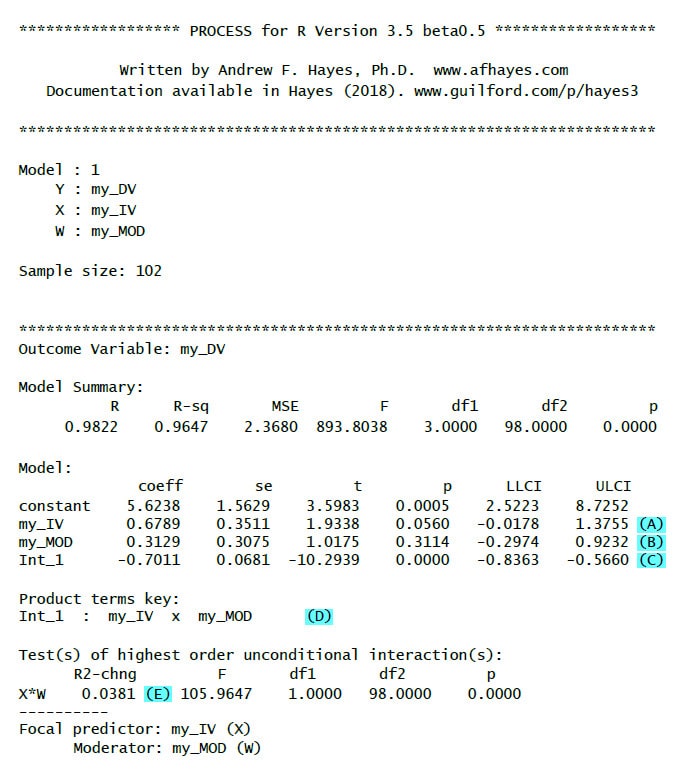
(A): Unstandardized regression weight (b) for the IV with test statistic, p-value and confidence interval
(B): Unstandardized regression weight (b) for the moderator with test statistic, p-value and confidence interval
(C): Unstandardized regression weight (b) for the interaction with test statistic, p-value and confidence interval. If this is significant then there is a moderation effect.
(D): Key for the interaction term (really important only for models with more than one interaction)
(E): R2-chng: Effect size of the moderation (how much additional variance is explained by adding the interaction term to the model)
(F): Effect (=b, second column) of the IV on the DV for a low value of the moderator (16th percentile, first column) – simple slope
(G): Effect (=b, second column) of the IV on the DV for a medium value of the moderator (50th percentile = median, first column) – simple slope
(H): Effect (=b, second column) of the IV on the DV for a high value of the moderator (84th percentile, first column) – simple slope
6. Additional Parameters
Even though the limited code above gives you the moderation test in many cases you want to have additional information. Following are some additional PROCESS parameters that could be helpful for your test whether there is an interaction.
Mean Centering
In a moderation analysis the interpretation of the regression weights is easier if you mean center the moderator (and maybe the independent variable, too). If you use set the parameter center to 1 all variables that go into interaction terms (IV and moderator) are mean centered. If you set it to 2 instead then only continuous variables are mean centered. Since mean centering of binary variables makes the interpretation of the results more difficult I only use this second value.
Example:
center = 2
Changing the Values for Interaction Probes
By default, interaction plots and probes are calculated for the median, the 16th and the 84th quantile. You can change this to – 1 SD, mean, + 1 SD instead (which I prefer) by setting the moments parameter to 1.
Example:
moments = 1
Significance Regions Johnson-Neyman
To get significance regions (Johnson-Neyman) you set the jn parameter to 1. I am using this setting when I have a continuous moderator but not with a binary moderator.
Example:
jn = 1
Plotting an Interaction
If you have a significant interaction it is helpful to plot simple slopes (i.e. regression slopes for different values of the moderator). You can generate the data for an interaction plot by setting the plot parameter to 1.
Example:
plot = 1
For me in R (in contrast to PROCESS for SPSS) that is not very helpful because I would have to write R code to generate a plot from this data. Therefore in case of a significant interaction I prefer using R packages to generate an interaction plot directly from the data, https://cran.r-project.org/web/packages/rockchalk/vignettes/rockchalk.pdf, see chapter 4.1 (Interaction in Linear Regression).
This would be a code example for plotting the simple slopes:
(First, you have to install the rockchalk-package with install.packages("rockchalk").)
library(rockchalk)
my_fit <- lm(my_DV ~ my_IV * my_MOD, data = my_data_frame)
summary(my_fit)
plotSlopes (my_fit, plotx ="my_IV" , modx = "my_MOD", modxVals = "std.dev." )
Including Covariates
If you want to add covariates to your model you can use cov =... If you have only one covariate you can simply put it into the formula. With more covariates you have to bind them together with c(....).
Examples:
cov = "age"
cov = c("age", "gender")
Bootstrapping
If you want to get robust confidence intervals for your estimates you can do that by setting the modelbt parameter to 1. Otherwise you would have to test the normality assumption before reporting any test results
Example:
modelbt = 1
Number of Bootstrap Samples
By default, for models with bootstrapping the number of bootstrap samples is set to 5,000. You can change this value by setting the boot parameter to the number of samples you would like to have.
Example:
boot = 10000
Bootstrapping - Start Value for the Random Numbers Generator
Bootstrapping has a random component. Based on a random numbers generator many random samples are being drawn from your data with replacement. As a consequence, if you repeatedly run an analysis with bootstrapping you will get slightly different results (p-values, SE, confidence intervals) each time you run the analysis. If you want to get the same results for each time you run the analysis you can give the random number generator a start value by setting the seed parameter to any integer number. (It is not important which number you choose.) Unfortuantely, still you will not get the exactly same results as when running the identical model with the identical data with PROCESS in SPSS because the random numbers generators of SPSS and R are different.
Example:
seed = 654321
7. My Favorite Moderation R-Code
The following code example for a moderation with two covariates (my_COV1, my_COV2) shows the options I tend to use when testing a moderation model:
process(data = my_data_frame, y = "my_DV",
x = "my_IV", w ="my_MOD",
model = 1, center = 2, moments = 1,
jn = 1, cov = c("my_COV1", "my_COV2"),
modelbt = 1, boot = 10000, seed = 654321)
8. Sample Output 2 – Moderation with Additional Options
Here an example of the output you should get with those additional options with comments only for the additional output elements:
(I): Regression weight for the first covariate with test statistic, p-value and confidence interval
(J): Regression weight for the second covariate with test statistic, p-value and confidence interval
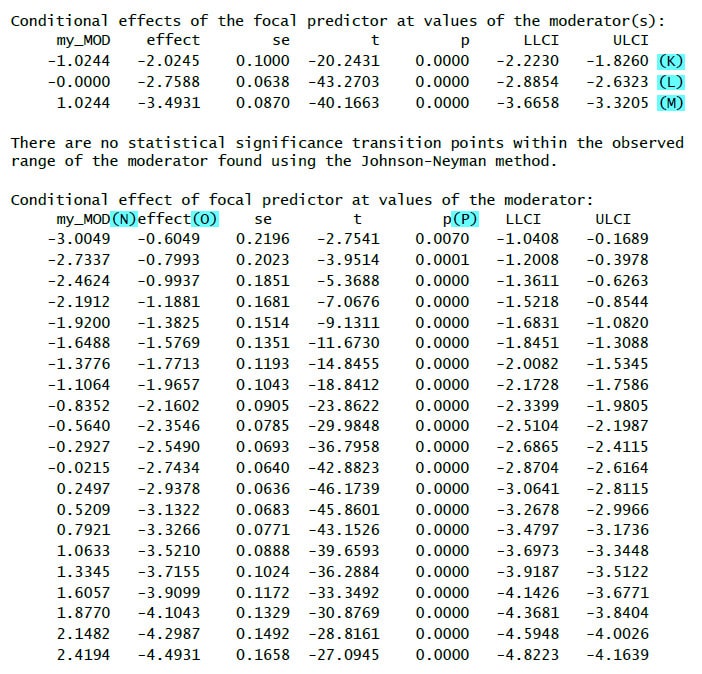
(K): Effect (=b) of the IV on the DV for a low value of the moderator (1 SD below mean) – simple slope
(L): Effect (=b) of the IV on the DV for a medium value of the moderator (mean) – simple slope
(M): Effect (=b) of the IV on the DV for a high value of the moderator (1 SD above mean) – simple slope
(N): Different values of the moderator
(O): Conditional effect (b) of the IV for the value of the moderator
(P): Significance test for the conditional effect
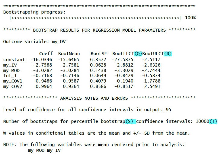
(Q): Lower limit of the bootstrap confidence interval
(R): Upper limit of the bootstrap confidence interval
If the zero does not lie inside the confidence interval (i.e. both limits are positive values or both limits are negative values) then the bootstrap results show a significant effect.
(S): Used bootstrap method (percentile bootstrap)
(T): Number of bootstrap samples (based on your chosen value for the boot-paramter)
9. More Information
If you want to know more about the theory behind a moderation analysis I recommend Andrew Hayes' excellent book:
“Introduction to Mediation, Moderation, and Conditional Process Analysis: A Regression-Based Approach”
http://www.afhayes.com/introduction-to-mediation-moderation-and-conditional-process-analysis.html